How Fast Is The Jet Propulsion Laboratory's Station Moving?

Concepts

The crust in Southern California is constantly moving and deforming
GPS receivers in the SCIGN network can measure these movements, even when they are very small
By collecting data over time, the movement of GPS receivers can be calculated
These movements are plotted on a graph, called a time series
The slope of the line connecting the data points represents the site's velocity, or rate

Materials

Pencil
Calculator
Print out of the time series for the GPS station located at the Jet Propulsion Laboratory (JPLM). This plot can be obtained via the SCIGN Analysis Homepage, located at http://milhouse.jpl.nasa.gov/scign or on the CD.

Required skills

Ability to read graphs
Basic knowledge of Trigonometry
Knowledge of rates

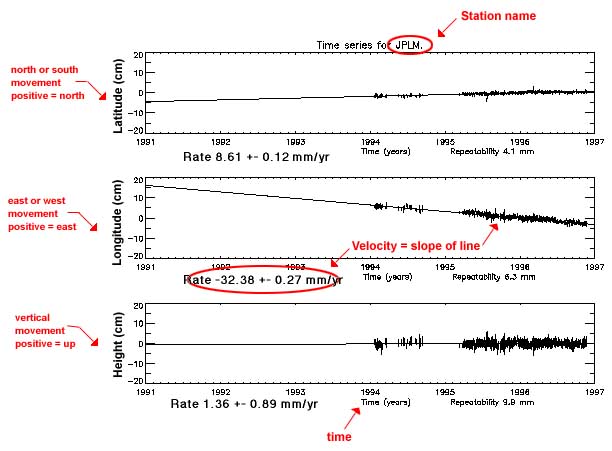
Background

The Southern California Integrated GPS Network (SCIGN) is a series of GPS receivers that continuously record information transmitted via radio waves by 24 satellites orbiting the earth. This information is collected and processed by scientists at JPL in order to determine the receivers' positions every day. This data is then plotted on a graph called a time series, which shows an individual receiver's position (y-axis) over time (x-axis.) By fitting a line to the data points and calculating the slope of the line, the velocity (a change in distance over a change in time) of a station can be determined. The time series supplies the calculated velocity for each of the position coordinates (latitude, longitude, height,) including error. If the slope were not supplied, it could still be determine by taking the rise (movement in one direction) over the run (time.) The time series also gives the station name, and the repeatability, the average change in the position over the total time.

Scientists can use this information to determine how a station is moving and simultaneously deduce what deformation is occurring in the Southern California crust. This is helpful in pinpointing areas that are deforming (straining) faster, which may mean an increased seismic risk. Hopefully, in the near future, the models made from the data collected by the SCIGN network will assist in determining aftershock risk areas following major earthquakes; lead to preventative measures limiting the destruction of buildings and property and advance the understanding of the earthquake process in Southern California.

Time series of all the SCIGN stations can be obtained via the SCIGN Analysis Homepage, located at http://milhouse.jpl.nasa.gov/scign

Helpful Formulas

Pythagorean theorem: D = (Dx² + Dy²)^1/2

Procedure

Below is a plot of the JPL station, JPLM. Examine the figure, and answer the questions following the plot. Click on the image to see a larger version.

1. What is the station name?

2. What is the latitude rate?

3. What direction is that?

4. What is the longitude rate?

5. What direction is that?

6. What is the vertical rate?

7. What direction is that?

8. How long has this station been recording data (according to the plot)?

9. What can you say in general about this station?

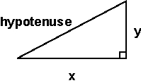
Challenge:

1. Using the rate values found in questions 2 and 4, for the latitude and longitude, and the Pythagorean theorem, solve for the overall horizontal velocity of the station (the hypotenuse.)

2. Now try the same calculation on another station of your choice (see URL in Materials section for additional time series.)

Questions to Answer

Why is it important to know how a GPS receiver is moving?
If a GPS station is moving, what else is moving?
Why should data be taken over a long time period?
How is having a network of GPS receivers, like SCIGN, helpful?
What might cause the tiny movements GPS receivers record between earthquakes?

What is SCIGN? Who runs it? Who has access? What happens to SCIGN data? How are the SCIGN data used? More about SCIGN
SCIGN Activities || Back to top